Tuesday, January 20, 2015

g force

No, not that kind of G-Force!

I mean the extra "weight" we feel pressing us down onto the bike or into the track when riding at speed around the curved banking of a velodrome.

If you really want to read up on g forces, then this Wikipedia page covers it.

First of all, "g force" isn't really a force, rather it's a measure of a rate of acceleration. It's one of those slightly confusing expressions.

g force is a way to "normalise" accelerations relative to that we experience every day due to gravity on the surface of the Earth. It's a way to gauge how much we'd "weigh" when experiencing an acceleration that's more or less than 1g.

When we are standing on the ground, we experience 1g (units are usually expressed a "g", not to be confused with grams). We are not actually accelerating, since the ground is there to stop us from falling, so instead we feel a force we call weight.

While we normally use standard international unit of metres per second squared (m/s^2) to express accelerations, it's common to express accelerations relative to that we experience on the surface of the Earth, which is defined a 1g.

If you have a mass of 80kg and are standing on the ground then you'll weigh 1g x 80kg. That's why many confuse weight with mass. They are not really the same thing, mass is an intrinsic property of an object, weight is the force it pushes down on the ground with. It's just that on when sitting on the surface of the Earth, an object with a mass of 80kg will also weigh 80kg.

However if you are accelerating upwards away from the Earth's surface (imagine you're travelling upwards in a rapidly accelerating elevator or rocket), then you'll experience more than 1g.

How much more depends on the rate of acceleration. If you happens to be accelerating upwards at 9.81 metres per second per second (which equals 1g), then you'd experience 2g, being acceleration due to gravity + the extra acceleration of the elevator or rocket. If you were able to stand on some bathroom scales while that acceleration is happening, then you'll "weigh" 80kg x 2g or feel like you now weigh 160kg. ugh.

Now keep in mind that an acceleration can be a change in speed and/or direction.

e.g. when a travelling in a car that turns around a corner, even through the road speed of the car may not change, we experience what feels like a force pressing us towards the opposite side of the car. Such lateral accelerations can also be expressed relative to 1g. Modern Formula 1 racing cars for example are capable of generating lateral corning accelerations of up to 6g.

g force on a velodrome


So whenever we are riding around the curved path on the turns of a velodrome, we are constantly accelerating towards the centre of the track, even though we may not be changing the bike's forward speed. As a result, we experience some lateral g forces when riding on velodrome, as well as the downward 1g due to gravity. What this means is the total g force we experience will be more than 1g. How much higher depends on our speed and the turn radius.

Calculating the rate of lateral acceleration when riding around a track is a pretty simple:
where:
- rider speed is in units of metres per second 
- 9.81 is the rate of acceleration due to gravity in metres per second squared
- rider turn radius is measured in metres

Estimating rider turn radius


To estimate a rider's turn radius, we start by estimating the track's turn radius.

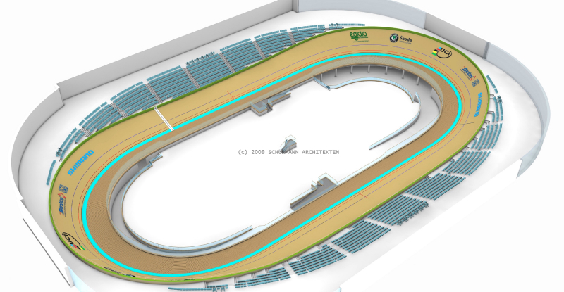
First an overhead shot of a velodrome to get a sense of the general shape of a track (thanks to Google maps). This one happens to be a local outdoor track not far from where I live. It's a 333.33m concrete track. You can make out the faint blue band around the inside of the track, which is just inside of the track's black measurement line, the inner edge of which = 333.33 metres in length.
Now we can approximate the shape of the track as being two semi-circles joined by two straights. Here I superimposed some circles and lines to demonstrate:
Of course tracks are not exactly like this, in reality the shape of the turns are not perfectly circular, and the length of straights varies. They really do come in many different configurations. But as an approximation you can see from the diagram it's pretty good starting point. So to make a reasonable approximation of a track's turn radius at the black measurement line, all we need to know is the total length of the track, and the length of the straights.
Let's say you are riding a 250 metre track with 44 metre long straights. The turn radius around most of the turn will be approximately (250 - 2 x 44) / (2 x PI) = 25.8 metres.

Like I said, it won't be exactly that as in reality tracks have a variable turn radius but it's close enough for the purposes of this discussion. OK, that's great, we have the track's turn radius.

Now back to our lateral g force formula:
Now this formula asks for the rider's speed and turn radius, not the track's turn radius.

The rider's speed and turn radius is based on the position of their centre of mass (COM). Since a rider leans over when riding around the banked turn of a velodrome, then their COM speed and turn radius is less than the wheel's speed and the turn radius at the track where the tyre is rolling along.

Another diagram to help explain. You might need to look at a larger version - so click or right click on it to view a larger pic. ('The pic of a leaning rider I found on this blog item. Hope they don't mind me borrowing it - I can't however vouch for the physics discussed in that item).

When a rider at speed rides around the turn of a banked velodrome, they are leaning over. That means the turn radius of their COM is less than the turn radius of the track where the tyre is rolling along. So if you want to calculate the g force on a rider you really should be using the COM turn radius and speed, which is a bit of a pain because bikes use speed sensors that measure the wheel's speed.

To calculate COM radius and speed, you then need to know the rider's COM height and their lean angle (from the vertical). It's a little basic trigonometry. 

e.g. if a rider's COM is 1 metre (COM height will be about the same as floor to saddle height for a rider in an aggressive race position), and they are leaning over at 40 degrees from the vertical, then the rider turn radius = track turn radius - sin(40 degrees) x 1 metre. IOW we reduce the track turn radius by ~0.64 metres, which for our 250 metre track is about 2.5% of the track's turn radius. So not much, but enough that for some applications and analysis of track cycling data you need to take these things into account.

That then brings us to the question of how do we calculate the rider's lean angle? Well I'm going to leave that one for now because I'm getting further away from the issue of g forces than I'd really like. Suffice to say that we can reduce the estimated track turn radius and wheel speed by a couple of percent to estimate rider turn radius and rider COM speed.

Are you still with me?


OK, so we can reasonably estimate the lateral g force of a rider travelling around the turns of a track. But of course the rider also feels the force of gravity pulling them downwards. So the total g force acceleration into the track is the sum of those two acceleration vectors:
Which can be expressed as follows:

So there you have it.

How much g force does a rider feel in the turns?


If we use an estimated rider turn radius of ~25 metres for a typical 250 metre track with rider speeds ranging from 40km to 75km/h, here's what the estimated g forces are:
At elite hour record speeds of between 52-55 km/h, a rider will experience around 1.3g to 1.4g when riding the turns.

There is a physiological question to be considered, namely does this higher g force, which occurs twice per lap and lasts for about 2/3rds of the total time on track, cause any problems with blood circulation, is it sufficient to hamper performance?

I don't know, and I'm not sure if there's been anything more than speculation on this question. 1.3-1.4g doesn't sound like it'd cause too much of a problem to me, but who knows?

Track sprinters


Things get much more interesting for the world's best track sprinters, who experience around 2g in the turns during their flying 200 metre time trial. If you have a 95kg track sprinter flying around at 75km/h, the bike, wheels and tyres are supporting the equivalent down force of over 200kg.

This is why track sprint bikes and wheels have to be made extra strong, and also partly why track sprinters run extra high pressure in their specialist tubular tyres.

Would you put a 200kg rider on your bike?

Read More......

Monday, January 19, 2015

Some kilometres are longer than others

With the spate of attempts at the UCI world hour record over late-2014 and into 2015 due to the revised UCI rules making the record within reach of more riders, it has naturally sparked interest in discussing what matters for best performance in the event.

Jens Voigt started the latest round of hour record attempts at the UCI's Aigle track
I recently saw some chat on a triathlon forum speculating about who could do what distance and so on. All in good fun, but none of them actually go to a track to find out. If they did, they'd realise it's not quite as simple (or as hard) as they might make out.

It pretty much comes down to optimising four main elements:
  • maximising sustainable power output for an hour
  • minimising the physical resistance factors of riding on the track
  • technical execution / skill
  • logistics & resources
Some might add psychological factors to that list, but ultimately I consider these to be expressed within the outcomes of each of the above.

Regarding logistics, there are of course UCI requirements to be permitted an official attempt an hour record, e.g.: minimum time in anti-doping bio-passport program is mandatory at elite level or dope testing at age group level, application submitted in advance for approval to relevant levels of cycling administrations, all the technical requirements including international level commissaires to supervise, a UCI approved track, use of timing equipment, start gates, specified date and time of attempt, etc. You can't just rock up and ride whenever you like. Well you could but it would never be a sanctioned attempt.

Then of course you need to factor in enough solo rider time on track for preparation, and that costs money and time as well. Quality indoor tracks are not always local, and even if they are, getting solo time on the track is not always so easy, let alone cheap. For an elite professional rider whose job is to race on the road, it may be difficult to devote sufficient time to the task of preparing properly for a track event.

Of course assuming the paperwork is all in order and you can do your training, then sustainable aerobic power and aerodynamics are king and the rider's ratio of power to aerodynamic drag area is the single most important factor for how far they will go in the hour. But W/m^2 is not the only factor.

There are other physical resistance force factors, like the influence of air density which is a function of altitude, temperature and barometric pressure (and to a much lesser extent, humidity) and the rolling resistance of the track and tyres chosen. I discuss some of these in the following items:
Altitude and the Hour record Part I
Altitude and the Hour record Part II

Which leaves us with technical execution and skill factors, of which there are a couple of key items, namely:


Riding good lines


Riding a good line involves a couple of components, one is pretty obvious and involves not riding further than you need to around the bends. Ride wide and you ride further. Pretty simple given the track is all but two semi-circles joined together with two straight sections. OK, the actual shape of tracks are more subtlety curved but that's close enough to describe why riding wide adds distance to your travels around a lap.

Design of the Glasgow Velodrome

If you ride 10cm wider in the turns, you add 10cm x 2 x PI = 62.8cm per lap.

If the extra width is measured on the track's surface, well the actual addition to the distance the wheel travels is reduced by the cosine of the banking angle. e.g. say the track's turns are, on average, banked at 40 degrees, and you ride 10cm above the black line. Then the actual additional track radius ridden is cosine (40 degrees) x 10cm = 7.7cm, and the additional distance per lap = 7.7cm x 2 x PI = 48.1cm. Nearly half a metre.

Do that over 200 laps or so for an elite hour record and you'll ride ~100 metres more than you need to. And that's for riding only a hand's width above the black line.

London Velodrome used for the 2012 Olympics
Another more subtle ride line factor involves the shape and design of the banking and in particular the transitions from the straights to the turns and back again, and whether it's advantageous to ride a slightly wider line in the straights to aid the transitions. On the straights you don't suffer the same severe distance penalty of riding a wider "radius" as you do when riding wide in the turns, so you can explore marginal gains in this manner.

However there is no simple or single answer to this, it depends on the rider and the track geometry - all of which have subtle differences. This is a somewhat more complex optimisation problem and I'm not going to delve into it here.

So putting aside these subtleties, the shortest distance around the turns is to ride the track's black measurement line* - ride any further out from the black line and you ride more distance each lap than is necessary. For the hour record you only get credit for the official lap distance each lap, which is typically 250 metres per lap on most modern standard indoor velodromes although some tracks are shorter and some are longer.

* it is possible to ride inside the black line, however in such timed track events like the hour there are foam blocks placed around the inside line of the track to ensure the riders don't. Very skilled riders can however ride fractionally under the black line on some tracks but it is risky as hitting the foam blocks can disrupt your effort and wash off some speed. The shape of the track in that small space between the black line and the wide blue section varies from track to track and it can be good or not so good to ride in.


Foam blocks discourage riders from riding inside the black measurement line.

Now why are some kilometres longer than others?


Office distance for the hour record =
(Official lap distance)  x  (Number of full laps completed within the hour)
+ a pro-rata distance calculated for the final incomplete lap

I won't go into the formula used by the UCI to calculate the pro-rata distance of the final lap (that's actually deserving of a blog post on its own as the regulations are remarkably confusing).

It matters not how far you actually ride, you'll only be credited with the official minimum lap distance per lap. This is why track riders and coaches are focussed on lap times and not with bike speed, since lap times are the integral of all performance elements. Power meter and other data loggers are of course valuable in parsing out the individual elements of performance that go into attaining lap times, and helping to prioritise development opportunities.

How good are riders at riding the minimum distance necessary?


It varies. Quite a lot. Skilled track riders are typically much better, which is what you'd expect. But what sort of penalty would an unskilled rider face if they started out on a track effort?

Of course we can do lots of maths to figure out how much extra distance on average a rider might cover if they ride wide by so much, but in reality riders move up and down the track, sometimes riding a good line, other times not so good. Some riders are just better at it than others and some adapt to the track more quickly than others.

It'd be so much better if we could simply measure what people actually do rather than speculate.

Which had me thinking. I have some data like that already...

Not so long ago I was doing some performance testing involving half a dozen pro-continental road racers at an indoor 250m velodrome. One of the features of the data logging system used for the tests is an ability to calculate the distance ridden per lap using the wheel's speed sensor data combined with track timing tapes to know precisely when they pass a specific points on the track. With some clever maths this is enough to nail the actual distance ridden each lap to high precision.

In amongst the test data were some solo efforts of at least 10% of the distance of an elite hour record attempt (i.e. 20+ laps of consistent effort) and several such runs by each of the six riders. I figured the runs needed to be long enough to reasonably approximate what a rider might be expected to do over a longer distance/duration.

Of course absolute accuracy of the distance the wheels travel depends on having an accurate wheel circumference value and that value not changing a lot while riding. So I'm not going to assume that the absolute accuracy was perfect, even though the absolute error might typically be somewhat less than 1%. More than that would require an error in tyre circumference assumption of 20mm, which is a lot for those used to measuring such things. However in our favour is that even if such an error existed, it would be a consistent bias error.

So rather than concern myself with absolute accuracy, I thought I'd compare the measured average lap distance for each run with the shortest recorded legitimate lap. In this way if there is any bias error, it's impact on this analysis is minimised (i.e. both measurements would be out by the same proportional amount). By legitimate lap, I mean a full lap not ridden below the black line.

Here's a table summarising data collected from the six riders (in no particular order). Each rider has multiple runs although I haven't identified the riders in the table. What the first column shows is the average lap distance per run less the minimum legitimate lap distance for that same run. The distances are of course distance travelled by the wheel.


Now the riders possibly could ride a tighter line than they actually did for their shortest legitimate lap, meaning that these distances likely underestimate the extra distance ridden when compared with riding very tight to the black line.

For the moment though let's assume the shortest lap they rode during each run was the best they are capable of doing. Since they actually did it, I think that's a reasonable assumption.

The average extra distance ridden per lap varies from one rider to another. One rider consistently rode only 0.3-0.4 metres more per lap than their shortest distance lap, while another was consistently riding more than 2 metres extra per lap on average compared with their shortest legitimate lap. The rider with smallest extra distance per lap had a track racing background.

The second column shows what that average extra lap distance would mean if extrapolated to riding 200 laps of a 250m track (an official distance of 50.000km). For one rider they would be riding nearly half a kilometre further than their track skilled team mate. Yet if both completed exactly 200 laps in the hour, each would be credited with riding precisely 50km, even though one rider's wheels had travelled nearly 500m further than the other's.

In this case, 50.5km = 50.0km. Some kilometres are longer than others.

So what's that extra 500m cost in power terms?


Well for a rider with a CdA of ~0.23m^2, that extra 500 metres travelled requires they output ~11-12 watts more than if they were able to ride a a better line.

Or they'd need to find a 3% reduction in CdA to make up for their skill deficiency.

Remember these were well skilled, well trained and experienced pro-continential road racers and finding an extra 10W or losing another 3% of aero drag coefficient isn't such an easy thing to do.

So no matter your current skill level and experience, if you're expecting to ride such an event yet you have never trained to become proficient riding on the track, well you might want to chop half a kilometre or so from your estimated distance covered based on your power and aero data alone.

Better still, just get to a track a find out what you can actually do.

Likewise, when estimating power, or W/m^2 from the official hour record distances, you might need to add some watts for the technical proficiency of the rider. The less proficient, the more power is required to attain the same official distance.


Read More......

Sunday, January 04, 2015

Accelerating Sins - Crank velocity variability

A few days ago I posted this item about the nature of how we apply power while pedalling and what impact this has on the variability in crank rotational velocity during steady state cycling, i.e. cycling along at a steady speed and power.

Part of the reason for examining this, other than for the sheer geek-out fun of it, was to assess whether the variability in crank velocity would violate a key assumption made by most crank/pedal based power meters used to calculate power, that assumption being crank rotational velocity doesn't vary during a pedal stroke, or at least not enough to impact accuracy.

Given the highly variable pulsing sinusoidal-like manner in which power is applied during a pedal stroke (something that has been consistently shown by published scientific measurements of pedal forces since the late 19th Century), then clearly some crank rotational velocity variation during a pedal stroke will exist. However due to the inertia of the bike + rider system, these variations are not typically large if you are using circular chainrings. It's a bit like how a flywheel is used to smooth out the power delivery of an internal combustion or a steam engine.

After discussing a little empirical knowledge and published research, I then examined a few scenarios with a modelling technique known as forward integration.

The outcome of that was, in summary; during steady state cycling at regular riding speeds and power outputs whilst riding outdoors, provided the chain ring is circular, then the amount of crank velocity variation is:
- mostly a function of the inertial load of the system,
- typically pretty small, and
- insufficient to cause concern for power meter accuracy.

However, as crank inertial load reduces significantly (e.g. at low speeds and high power outputs, or when riding on a very low inertia inddor trainer or one with unrealistic resistance) the level of crank rotational velocity variation may begin to introduce some small level of inaccuracy in reported power.

The issue of chain ring shape and the resulting increased variability in crank rotational velocity and associated error in power measurement it introduces to crank/pedal based power meters has been discussed by others, including on Tom Anhalt's blog and Dan Connelly's blog, so I won't go through that here.

OK, that's for steady state cycling. What happens when we are accelerating?


Obviously if we are accelerating, then the crank's rotational velocity must be changing as well. Not only with the trend of overall increase in speed of the rider, but also it will vary up and down about that general increase in speed trend.

So just how much variability in crank rotational velocity is there when accelerating?

I know there are some labs that have actually measured this stuff, but for now I don't have access to such data, so I thought I'd do some more modelling using first order approximations as described in my post the other day, and apply it to an acceleration scenario I have previously modelled.

In December 2014 I wrote Sum of the Parts II, which used similar modelling to compare accelerations with each of two wheel-sets, one that was lighter and less aerodynamic with another that was heavier but more aerodynamic. In that case the aero wheels win just about all the time.

But it had me thinking, as well as another anonymous person who commented on the Sins of Crank Velocity post, what does the bike speed and crank velocity variation look like when accelerating?

So, I thought I'd have a go at modelling it. Great. Now things start to get a little complicated.

First some assumptions:

Assumption 1. 
I'm going to use the power output profile as described in The Sum of the Parts II blog item for a 10-second sprint from a start speed of 30km/h. Here's an image which shows the power curve and speed line that results. It's ~1000W on average but with a power output curve as shown by the yellow dashed line below:


Power starts at 250W, rises quickly to ~ 1250W and then fades through the remainder of the sprint. The rider we can see accelerates from 30km/h to 51km/h. That's a slightly faster end speed than the previous blog post showed, mainly because I'm using a slightly lower value for assumed CdA (aero drag coefficient) in this model (as that's what I used in the crank velocity variation model I highlighted on 1 January).

Given the way power is actually applied in a pulse-like manner, then the real power curve is not as smooth as shown. This is really just a plot of the overall trend in power over that 10-seconds.

Assumption 2. 
No gear changes during the acceleration. I'll assume a 53x15 gear, which is a gear ratio of 7.40 metres. For the track riders out there, that just a bit less than 50x14 gear (7.48m).

Assumption 3.
That power application during a pedal stroke follows a sinusoidal-like pattern but in this case with an ever decreasing period between crank rotations, IOW the cadence is constantly increasing through the acceleration in line with the bike's speed increase. As discussed in the previous item, this is a first order approximation, and the torque profile while accelerating hard will be different to that when riding steady state. We tend to engage our leg muscles differently and also use more upper body musculature in the action. Even so I think using a sinusoidal-like power curve is still a good first order approximation.

Assumption 4.
The model starts with the crank vertical and pedal at top dead centre, power drops to zero watts momentarily each time the crank is in this position - and the left and right legs can apply power symmetrically. Like I said, it's not intended to be a perfect model - just a first order approximation.


Now solving the problem of generating this variable power curve gets a little complicated, and I'm not going to attempt to describe how I did it, but let's just say that it required an iterative process.

Here are some plots to show what's going on. This is the power curve once I overlay a sinusoidal function onto it. It's not a standard sine wave, since the period for each crank rotation reduces as the sprint progresses, and the amplitude varies along with the general power output trend. As always, click on the image to see a larger version.


The basic principle of the peak power being double the average power for the pedal stroke is in line with expected torque/power profiles. As you can see the instantaneous peak power rises to a maximum of nearly 2500W and oscillates between the power peak attained during each down-stroke, and zero watts as the crank arm passes through top dead centre.

If you look at the two red arrows drawn on the bottom axis, you'll see each marks the time taken for the first and the final complete pedal stroke during the 10-second sprint. This is to highlight the ever reducing time period between pedal strokes as cadence increases along the way.

The first full pedal stroke takes 0.87 seconds (69rpm), and the final one 0.53 seconds (114rpm).

Now to overlay the resulting speed curves:


The above plot show 4 lines:

  • The smoothed power trend line (dashed yellow)
  • The instantaneously variable power line (unbroken yellow) as applied to the cranks
  • The smoothed speed trend line (dashed blue)
  • The instantaneous speed line (unbroken blue) resulting from the application of variable power 

Here it is without the instantaneously variable power line so you can more easily view the resulting speed plot:


You can see that the actual speed curve oscillates about the general trend line, and that it varies more at the start of the sprint than it does at the end.

Let's zoom in to see this a little more closely. Here's the first 2.5 seconds, with the speed axis zoomed in some more to amplify the variation:


Power rises and falls rapidly, and reaches an maximum instantaneous peak of just under 2500W (actual peak occurs at 2.55 seconds). Thereafter power plateaus and fades.

Here are the final 2.5 seconds of the acceleration with the same level of speed scale zoom:


Power in the final 2.5 seconds fades to a trend average of ~660W at the end of the 10-second acceleration

If you look at the speed plots in each, it's pretty clear the level of speed variation, and hence crank rotational velocity variation, is much greater during the early phase of the sprint when speed is lower and power is higher, and the variability reduces as speed rises towards the maximum.

So how much variation is there?


Summarising the difference in crank velocity during the initial and final pedal strokes:

So the variability in crank velocity for this hard acceleration is greatest in the first few pedal strokes, but then begins to reduce as speed increases, reducing to just +/- 0.2% by the end of the effort.

Impact on power meter accuracy?


Given the size of the crank velocity variance, then it's possible there may be some inaccuracy in reported power. Let's examine one revolution of the crank during the early phase of the sprint to get some idea of what's going on. Here's a zoomed in chart with four lines plotted (click on image to see larger version):


The non-shaded area represents one complete crank revolution - in this case I've chosen the start and end points at the point of peak power (yellow line).

Also plotted is the associated torque profile (red line) in Newton.metres.

Finally, instead of bike speed, I have shown crank velocity in radians per second. There are two speed lines shown, the instantaneous crank rotational velocity (lighter blue line), which varies throughout the pedal stroke, and the average crank velocity (horizontal dark blue dashed line) for that revolution (= 2 x PI / duration of crank revolution in seconds).

Actual Power


Now the true average power in this instance is the average of all the instantaneous power values. In this particular model I am performing calculations for every 1/100th of a second (in some models I use a greater frequency, others less, it depends on the precision needed). A 100Hz "sampling rate" seemed adequate for this purpose.

By averaging all the individual power values, the true average power of the complete crank revolution is 1119W.

What power meters report


However, power meters don't sample crank velocity more than once per crank revolution, they instead they calculate power as the average crank velocity x the average of the torque samples during that crank revolution.

In this case the crank revolution takes 0.770 seconds, which converts to an average crank velocity of 8.16 radians per second. The average of the torque "samples" during that crank revolution was 140.9N.m.

Hence power calculated this way = 8.160rads/s x 140.9N.m = 1146W

That's a difference of 27W, or 2.4%.

Now the variance between maximal and minimal crank velocity during that crank revolution was 4.6%, so we can see that the error in power calculation introduced due to the assumption of constant crank rotational velocity is about half of the maximal variance from the average.

As the sprint progresses, and the crank velocity variation reduces and speed plateaus, then the error in reported power will diminish significantly.

Standing start?


This modelled acceleration was from a rolling start (30km/h), so one might expect greater crank rotational velocity variance in the initial phases of a standing start. But modelling that is for another day.

Something else to keep in mind:


SRM power meters sample torque at 200Hz, hence during this hypothetical crank revolution an SRM would provide 154 individual torque samples, and also uses a magnet triggered electromechanical reed switch to obtain an accurate cadence timing point.

However many other power meter models sample torque at a much lower rate, e.g. 50Hz or 60Hz, meaning there are as few as 38 or 46 torque samples in that example pedal stroke) and some also use an accelerometer divined cadence trigger meaning the exact timing of each pedal stroke may not be as precisely defined and perhaps results in some aliasing of the reported stroke by stroke average crank velocity (cadence), and number of torque samples used.

As a result, power meters that have lower torque sampling rates and that use accelerometer derived cadence may not necessarily report peak power as accurately.

Read More......

Thursday, January 01, 2015

The Sin of Crank Velocity

Crank and bike speed variations during a pedal stroke


This topic occasionally comes up in discussion in cycling forums – just how much does crank speed vary during a pedal stroke? And how much does this affect the accuracy of power meters?

If you are pedalling along at a steady rate and maintaining a consistent power output (in other words you are not attempting to accelerate or slow down) and are using circular chainrings, then the short answer is: not a lot.

But crank rotational velocity during a pedal stroke is not totally constant, there is some variation.

Of course anyone who has ridden a bike behind a derny or motor pace bike on flat terrain or at a velodrome knows they are able to ride consistently close to the rear guard or roller of the motorbike and not experience significant fore-aft movements during each pedal stroke.

Riders following a motor pacer manage to remain very close
to the pacer and don't experience large fore-aft relative motion.

Riders in a highly skilled team pursuit formation riding at high power outputs are also able to ride within centimetres of the wheel in front without experiencing major changes in velocity between riders during each pedal stroke, which if it did happen would of course be somewhat disastrous. Note the riders below are all at different phases in the pedal stroke:

Track Cycling World Championships 2014: GB women's team pursuit team
Image from: www.telegraph.co.uk
So even without any examination of the research, or doing any fancy modelling of the physics involved, we already know empirically there really isn't going to be large variations in bike and crank velocity.

So how much variation is there and what influences bike and crank speed during a pedal stroke?


When pedalling in a steady state manner, the main factors influencing the variability of crank velocity are:

  • The average power being applied
  • The manner and level of power variation during a pedal stroke
  • The inertial load of the system (i.e. the speed and mass of the bike + rider, plus a little rotational inertia from rotating components)
  • The resistance forces in play (i.e. air and rolling resistance, gravity, and changes in kinetic energy) and whether for example air resistance is dominant (e.g. when riding on flat terrain), or overcoming gravity is dominant (e.g. climbing a steep grade)
  • The shape of the chainrings, or as in the case of some weirdo bike crank and pedal sets ups, the variable effective radius of the crank arms

Why do we care about crank velocity variation?


Apart from satisfying our curiosity on this somewhat esoteric matter, the answer does have a few practical applications with respect to cycling performance, one of which is to do with power meter accuracy. Others pertain to efforts seeking to eek out minor performance gains though examining mechanical adaptations to the bicycle drive train, such as design of non-circular chainrings. Whether these designs result in a performance improvement is debatable (the research is equivocal on the matter for sustainable aerobic power) and not the topic of this post, so I'll leave it there for now.

Power meter accuracy and crank rotational velocity


Many power meters, e.g. SRM, Quarq, Power2Max, Garmin Vector and Stages, rely on the assumption that crank speed during a pedal stroke does not vary (Powertap on the other hand assumes wheel speed does not vary during their fixed duration torque sampling period of 1 second).

This is an important assumption, since torque is sampled at a fixed frequency (e.g. at 200Hz for an SRM or somewhat lower, e.g. at 50-60Hz for other brands) and then those torque samples are averaged over a complete crank revolution. This averaging of torque over a full revolution to calculate power will only be accurate if the crank velocity does not vary much during the pedal stroke.

If however a rider pedals significantly more slowly during one part of a pedal stroke compared with another, then that slower part of the pedal stroke will be over-weighted in the average of total torque samples. Hence interest in examining the assumption about constant or near constant crank velocity during a pedal stroke.

So let’s look at some of the crank velocity variability factors I mentioned earlier.

Power application during a pedal stroke


It’s well known that when we pedal we apply torque to the cranks in a pulse-like manner, with each leg’s down-stroke moving from a phase of minimal propulsive power when the crank is vertical with the pedal at top dead centre, increasing propulsive force and power as the crank moves down towards the horizontal, and diminishing as the crank moves towards the vertical again with the pedal at bottom dead centre. It looks a little like this:
Image courtesy of:
http://www.rohloff.de/en/company/index.html
In steady state cycling we apply little if any propulsive force on the upstroke and some may in fact apply a little negative force (this is not necessarily a bad thing and is something often misunderstood about pedalling dynamics - but I digress).

This pulse-like power cycle is repeated by the opposite leg and crank arm, so that for each full revolution of the crank, we apply two pulses of power, mostly from the down-stroke push of each leg.

This pulsating nature of power application has been measured and is well reported in the scientific literature, and typically shows a wave-like sinusoidal pattern (i.e. it looks like a sine wave), which should come as no surprise given our legs act like two pistons pushing down on rotating crank arms.

Studies examining this go back many, many decades, e.g. this 1968 paper by Hoet at al as an example reported the following finding:


Those summary findings by Hoes et al have been consistently replicated in many subsequent studies.

Such analysis goes back even further, to the late 1800s. Pedal pressure was measured and shown in this book: Sharp, A. (1896). Bicycles and tricycles: an elementary treatise on their design and construction.

This fabulous old book (which covers a huge range of cycling physics and performance matters over 32 chapters and which Lee Childers at Alabama State University kindly referred me to) is available in scanned form online here:

https://archive.org/details/bicyclestricycl02shargoog

Here are image scans from four of the book's 561 pages showing pedal pressure measurements from various riding conditions on a fixed gear bicycle (flat track riding, ascending and even back pedalling when descending). Read from the bottom of page 268 - Section titled: 214 - Actual Pressure on Pedals.


The charts plot the measured pedal pressure, which is not the same as the tangential (propulsive) forces, a point made on page 270 - but even so we can see the basic shape of pedal forces follows this basic pattern. Indeed Sharp refers to such tangential pedal force measurement pedals designed by Mallard and Bardon, their "dynamometric pedals". I don't have a link to show these unfortunately. This was the late 1800s. What's old is new again.

Below is an image from the 1991 Coyle et al paper showing the measured crank torque applied by one leg through a full pedal stroke for each of the 15 riders in the study. We don’t need to inspect the plots too closely; the main point is we can readily see the approximately sinusoidal shape of torque applied to the cranks during the down-stroke phase, and the minimal torque applied during the upstroke phase.

The primary differences between riders are in the amplitude of the down-stroke phase of curve, and the shape of the upstroke phase, which mostly hovers around the zero line. As always, you can click on an image to see a larger version.


If you then imagine the opposite leg repeating the same type of torque application, then we can see we apply torque to the cranks in a pulsating wave-like, or sinusoidal, manner. This sinusoidal curve was also demonstrated in the 2007 Edwards et al paper which included the following plot of typical pedal torque applied by both legs for a full crank revolution:


So while not perfect sine wave-like application of torque, thinking of the force applied to the cranks as being sinusoidal-like is a very good first order approximation.

Users of indoor bike training systems like Computrainer, Wattbike or SRM's Torque Analysis System may have also seen similar torque output curves. Here’s a random example of an image of a Computrainer SpinScan plot I found with a quick Google search:


Now SpinScan is not as fine a resolution measurement tool as used in scientific study, but at least you can see that the same basic shape of the power output curve during a pedal stroke. Wattbike charts are typically displayed in polar chart format, so to avoid confusing things I won’t post a picture here but the same overall pattern of torque and power application is repeated, as they are with SRM's Torque Analysis system (although this is a very low power example from SRM's website):


One thing we can see with all these examples is how power doesn't generally drop all the way to zero while pedalling, and that it is often not symmetrical for left and right legs.

I have generated a sample sinusoidal power curve to reasonably approximate this pedal power pattern which I'll use for modelling I'll discuss later on. In this case it shows the power curve when pedalling with an average power of 250 watts at 90rpm (click on pic to see larger version):


Now this is by no means a perfect model of actual power application, and as can be seen from the various charts shown earlier, everyone pedals slightly differently, but it’s certainly a very good first order approximation to examine the issue of how much bike speed is affected by application of such a pulsating power curve. It matches the general shape of actual torque delivery delivery and the peak power is nearly double the average power, which also matches the torque profile measured experimentally many times, and at least since Hoet at al reported this in the 1960s.

Naturally the power curve is a function of both crank torque and crank velocity, but as we shall eventually see, the latter does not vary all that much, certainly not enough to make this first order approximation invalid for the purpose of answering this question.

So what effect does this pulsating variable power output have on bike and crank velocity?


Firstly I’ll look at an example of what’s actually been measured and reported in the scientific literature, and then I’ll examine the physics with some modelling.

Actual measurement of crank speed variations


Crank speed variations during a pedal stroke were reported in this paper by Tomoki Kitawaki & Hisao Oka: A measurement system for the bicycle crank angle using a wireless motion sensor attached to the crank arm, J Sci Cycling. Vol. 2(2), 13-19.

Here’s a link to a pdf of the paper I found in a Google search:
http://tinyurl.com/qapfoek

I'm referring to this paper in particular as it provides some helpful images and a full version is available online for anyone interested in examining it in more detail. Other studies have also measured crank velocity during pedalling and found similar results, but the data may not be available in the freely available public domain nor presented in such a convenient and helpful manner as needed for this discsussion.

Figure 6 of this study (shown below) summarises the measured variability in crank velocity over a range of power outputs for riders in three groups categorised as beginner, intermediate and expert level by their relative power to weight ratio being approximately 1.5W/kg, 2.25W/kg and 3W/kg respectively.

Crank velocity for each group is shown at two different cadences (70rpm and 100rpm) and was measured using two different crank velocity measurement systems (the study was primarily to examine the validity of a crank angle and velocity measurement system compared with a standard. As it turns out the two methods matched quite well). They also measured the crank velocity variations at the riders’ freely chosen cadence but did not provide charts for those data.


In this study, riders used their own bike on a CycleOps Powerbeam Pro trainer, which is a fairly typical and relatively low inertia indoor trainer.

It shows six charts. In each the crank rotational velocity relative to the average crank rotational velocity (i.e. the normalized crank rotational velocity) is plotted by crank angle for a complete pedal stroke. There are a series of dots and lines plotted in the charts, and these represent the normalized crank rotational velocity as measured using two different measurement systems.

The maximal variance in normalized crank rotational velocity occurs in the most powerful group of riders, and at the lowest pedal rate (70rpm). The variance in this case was around +/-3% and in all other cases the crank velocity variance was less than +/-2%.

Keep in mind this experiment was performed on a low inertia trainer. Why does this matter? 


It matters because a mechanical system (or an object) with lower inertial load will accelerate (or decelerate) more rapidly when a net force is applied to it compared with a system with greater initial inertial load. Many indoor trainers, like the Powerbeam Pro used in this study, have lower crank inertial loads for the same rear wheel speed compared with what a bike and rider riding out on the road typically possesses.

So what happens when we examine the case of a more realistic road-like inertial load scenario?


Since I’m unaware of published and validated crank velocity measurements readily available from actual on road riding (if anyone can point me to any please let me know), we can instead examine the physics of what happens to a bike’s speed when power is applied in this pulsing sinusoidal-like manner.

Forward integration - Balance sheet accounting for energy


To do that I use the technique of forward integration, a technique that’s really no more complicated than an accounting balance sheet but for energy rather than money.

On one side of the balance sheet is the energy supply coming via our legs, and the other side of the balance sheet is the energy demand, i.e. the power required to overcome various resistance forces such as air resistance, rolling resistance, gravity if changing height, and importantly resistance to changes in speed (kinetic energy). That energy balance sheet must remain in balance. It’s a fundamental law of nature.

At any point in time if we know a rider’s speed, their mass and that of their bike, the moment of inertia of their wheels, their coefficients of air and rolling resistance, the road gradient, and other small frictional loss factors, then we can calculate how much power is required for each of these various resistance forces, and when added together they tell us how much power is required to maintain that speed.

If a rider’s actual power output is different to that required to maintain the same speed, then the balance of power supply must result in a change in kinetic energy, and hence a change in speed.

If a rider is in deficit on the energy balance, then that deficit must come from somewhere and that means their kinetic energy (and hence speed) must reduce by the same amount accordingly. Put another way, they are not supplying sufficient power to maintain their original speed and must therefore slow down.

Conversely, if the rider is providing power in excess of that required to maintain their original speed then they will accelerate, and at a rate so that the increase in kinetic energy matches that energy surplus.

In the model these calculations are made for each brief moment in time, the net energy surplus or deficit for that initial speed is determined and converted to the exact change in speed required to maintain the energy balance.

Let’s examine what happens to a rider’s speed in a sample scenario.
250W, flat road @ 90rpm


Riding along at 90rpm on a dead flat road with no wind and with an average power of 250W at around 36km/h with:

  • Bike + rider mass: 80kg (including wheel rim mass of 1kg)
  • Coefficient of rolling resistance (Crr) of 0.005 (fairly typical for good road tyres on asphalt/chip seal surface)
  • Coefficient of drag area (CdA) of 0.35m^2 (e.g. road bike on the hoods)
  • Air density of 1.20kg/m^3 (sea level, 1020hPa, temp 21C, relative humidity 77%)
  • Drivetrain efficiency:  100% (just to keep it simple, although ~97% is typical)


Using the forward integration model with the simulated sinusoidal-like power output during a pedal stroke, we can now plot the impact on bike speed during a pedal stroke. Click to view a larger image.


In the chart above we have the power output (yellow line) varying during the pedal stroke, which takes a total of 0.667 seconds to complete each revolution. The plot show 1 full second of pedalling, and so the graph actually shows one and half revolutions of the crank.

The initial velocity is set to a little under 36km/h. The speed resulting from that pulse like power input is also plotted by the blue line with the left hand axis being speed. Note the speed scale ranges from 24km/h to 40km/h and so is already zoomed in a little to amplify the variation. At that slightly zoomed scale we can see that the speed line wavers up and down just a little during the pedal stroke.

Since it’s a little hard to see how much variation in speed happens, let’s zoom in much more by adjusting the speed scale to amplify that speed variation curve.


Note the scale of the speed axis on the left side – each horizontal grid-line represents 0.05km/h, and the variation in speed is easier to see.

When power is higher than that required to maintain a constant speed, then speed increases. Eventually though the power drops below the level required to keep accelerating, and speed levels off then begins to decline as power has dropped such that there is now an energy deficit compared with that required to maintain that speed, and so kinetic energy (speed) must fall. As a result, the speed plot follows a similar sinusoidal-like curve, but out of phase with the power plot.

Here’s a table summarising the average, minimum, maximum and amount of variation in power and speed.


The normalized speed variation is less than +/-0.2%.

As I said, not a lot of variation in bike speeds during a pedal stroke, even though the power is ranging from a low of 20W up to a maximum of 480W twice each pedal stroke.

That's bike speed - what about crank velocity?


Now the next logical step is to assume that this “all-but” constant bike speed is also matched by constancy of chain speed and hence crank speed. Since the chain is moving around the rear wheel's circular cog and the upper drive section of the chain has positive tension then that is what you would expect.

So provided the front chainring is circular, this will also result in a nearly uniform crank rotational velocity.

Hence in this steady state cycling scenario we need not be concerned with any inaccuracies in power measurement due to the assumption used by power meters that crank velocity is constant during a pedal stroke.

For crank velocity not to closely match the bike’s velocity it would require the part of the chain under constant tension to stretch and contract significantly during each half pedal stroke, or for the chainring to not be circular. Chains just don’t do that but chainrings may be all sorts of curved shapes.

Sensitivities and assumptions


As I said earlier, this input power model is only a first order approximation; people apply power slightly differently, and not necessarily symmetrically or consistently. Some of the other assumptions may not necessarily hold, e.g. aerodynamic and rolling resistance coefficients, and drivetrain efficiency remaining constant during a pedal stroke when they may in fact vary a little during pedal stroke. The rider’s legs also slightly vary their kinetic and potential energy as they move through a pedal stroke,

These are second and third order effects that would only make minor changes to the shape of the modelled speed curve, and we can see that the speed variation is already so small such that second and third order modifications are not going to change the outcome to any significant degree.

What about when climbing a steep hill?


When climbing, average speed for same power will be significantly less than when on a flat road. On an 8% gradient our 250W rider will be travelling at closer to 13km/h instead of 36km/h. That’s means a much reduced kinetic energy – which is dominated by translational KE of the rider.

KE = 0.5*mass*velocity^2,  plus a little bit from wheel rotational inertia (which is very small).

The translational KE of our 80kg bike and rider at 36km/h is 4,000 joules, and at 13km/h it’s 522 joules, or only 13% of the KE at 36km/h, even though velocity is 36% of flat road speed.

The next big difference is the resistance forces are now dominated by overcoming gravity rather than overcoming air resistance. This also has an impact on the size of bike speed variations during a pedal stroke, the result being we should expect changes in speed to be greater.

Finally, many riders have a tendency to pedal at a lower cadence when climbing steep hills. Not everyone does of course, but sometimes the available gearing means a lower cadence is inevitable. So for the sake of this scenario, let’s assume the rider’s cadence has dropped to 60rpm (that's about what cadence would be with a 39x23 gear at 13km/h).

This is the power and speed plot:


Since the cadence is 60rpm, it take a full second for each pedal revolution. We can see even with the low zoom level on the speed axis that the bike’s speed line does indeed vary more than when on the flat road.

Here’s what the speed variation looks like using the same zoomed-in view setting as before:


So when climbing there is a much greater variation in bike speed during a pedal revolution than when riding on a flat road at higher speed, but it’s still less than +/-2%.

Is a +/-2% crank speed variance during a pedal stroke something to be concerned with for power meter accuracy? 


As a rough rule of thumb, the error this would introduce to the calculation of power would be approximately 40% of the crank speed variation, or less than 1%. Whether that 1% error matters to you I can't really say, but it's a couple of watts and for most people it's not a significant factor for the purposes they might be using power meter data from climbs for.

If you are doing some aerodynamic field testing though, then such an error would be of concern. Fortunately we don't do such testing on steep climbs all that much, but rather mostly on flatter terrain where any error due to crank rotational velocity variation as we have seen is tiny.

That’s a 3.5W/kg rider. What about a more powerful 5.5W/kg rider climbing that 8% grade?


More powerful riders climb faster, and likely pedal at a higher cadence as well, so let’s assume our 400W rider climbs the 8% grade and pedals at 75rpm (that's roughly the cadence if pedalling a 39x19 gear at 19 km/h). This is the resulting power and speed plots:


So even though the rider is more powerful and has much greater variation in power output, the increased cadence and higher speed means the normalized crank rotational velocity variation is only +/-1%, and power meter error is likely to be less than 0.4%.

Summary


While pedalling in a steady state manner out on the road with circular chainrings, crank speed does not vary all that much. It varies more when climbing than when riding along flatter terrain, but the amount of variation is still small such that the basic assumption of non-varying crank velocity used by power meters to calculate power is sufficiently valid and within their generally stated margins of error.

Crank speed variation is larger when riding on low inertia trainers, such that the level of potential error in reported power may begin to approach the limit of the devices' stated error margins.

Read More......